Training of the neural network can be performed in three different ways represented by the three buttons at the bottom of the dialog window:
![]()
1.The Train Network button directly starts the configured training locally. Depending on the checkbox Use GPU, either your CPU or GPU will be used. Note that only the samples explicitly selected (left-click, ctrl+click, shift+click) in the 2. Samples list will be used for the training, according to the settings in 3. Training Parameters and 4. Preprocessing parameters. As a result, the weights and manifest files will be updated.
2.Using Export R workspace, the configured preprocessing operations are applied to the selected data and the resulting images are exported together with the training configuration in the form of a compact R workspace. The workspace can then be transferred to a more powerful processing environment for the actual training. This can either be another PMOD installation on a more powerful machine or in the cloud.
3.The Train Network with Workspace button opens a dialog window in order to load a previously exported R workspace and starts the training locally.
The process is described in detail below.
Deployment
After completion of the training, the resulting Weights and Manifest files are combined with the Learning Set definition (*.aiset file) to form the trained model. The trained model can be used in the same PMOD installation used for training by selecting the Learning Set from the database where AI functionality is available. The trained model can also be transferred to other PMOD installations for prediction. This is most easily achieved by using Export as Model and copying the resulting files from the PMOD installation folder resources/pai/architecture/weights (e.g. C:\Pmod4.4\resources\pai\unet_002\weights\IXI_Parcellation\) to another PMOD installation.
Recommendations
On typical personal computers local training is only recommended for tests with a limited amount of data. Performance may be acceptable with data that has a small matrix size (e.g. 50 x 50 x 50 for cropped PET data) and low number of input series for multichannel segmentation (e.g. 1 or 2). The total time required for training cannot be estimated. While training is running you will see a significant load on CPU/GPU and a plot of loss value by epoch in PMOD’s R Console. Even for powerful workstations, training with hundreds of samples may take many hours. Training on a cloud computing infrastructure with virtual machines accessing several GPUs is likely to be more time- and cost-efficient.
It is advisable to always perform a small "infrastructure check" training before launching training with your full data set and many epochs. This can be performed using the minimum requirement for input samples (2 samples), a batch size of 1 and a low number of epochs (1 is acceptable, but 2 or 3 will reveal changes in the loss value in the Manifest). If the input data has a high matrix size (e.g. 200 x 200 x 200) and/or there are multiple input series in the sample, the data volume could be reduced by using a larger pixel size for this training test (e.g. 2 x 2 x 2 mm instead of planned 1 x 1 x 1 mm).
Training Progress and Output
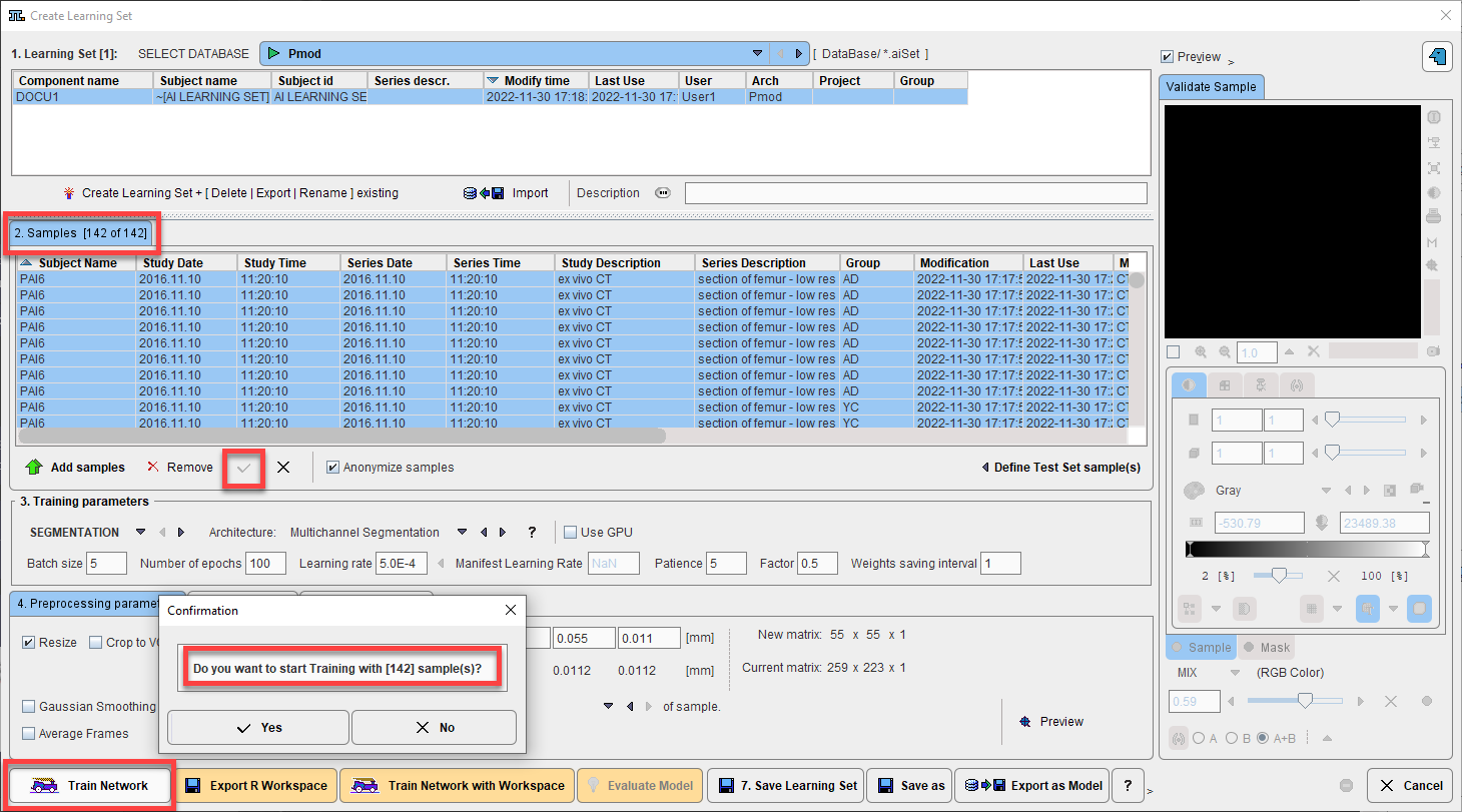
For data prepared on your local system, training is started by selecting the desired samples in the Learning Set and clicking Train Network:
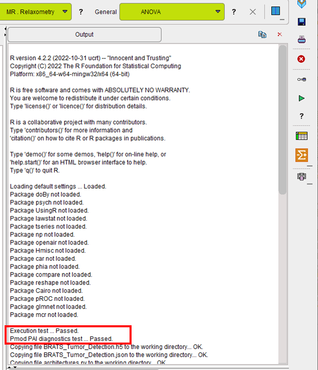
The RConsole opens and the Execution test and PAI diagnostics test are performed. If the tests are passed the selected samples (all input series and associated Segments) are loaded:
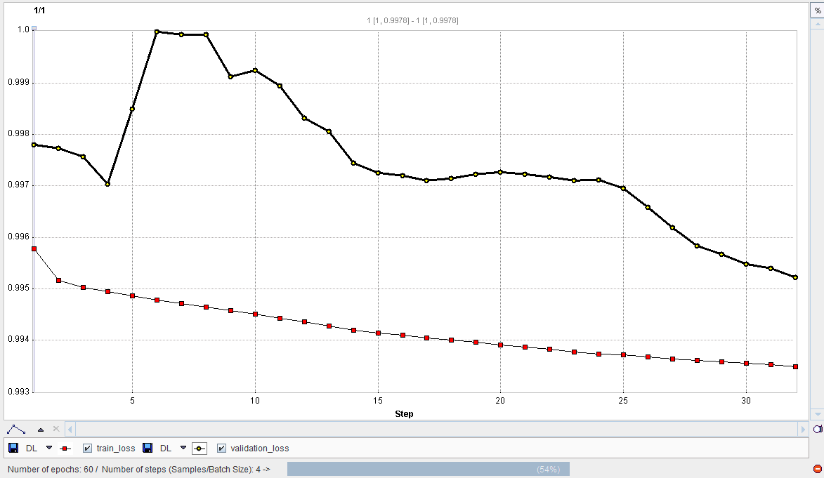
During training the loss value is plotted with each epoch. Note that the loss value depends on the architecture selected and large changes on the y-axis are possible. In the example shown the loss value is 1 - Dice Coefficient for training of the unet_002 Multichannel Segmentation architecture with rat brain dopaminergic PET data as described in our Case Study. At the start of training the loss value is 1, and successful training results in a reduction of the loss value towards zero:
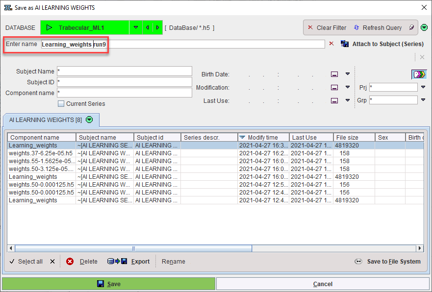
Once training is complete a dialog appears to save the Weights. They can be saved to the database or file system (the same database as the Learning Set is recommended):
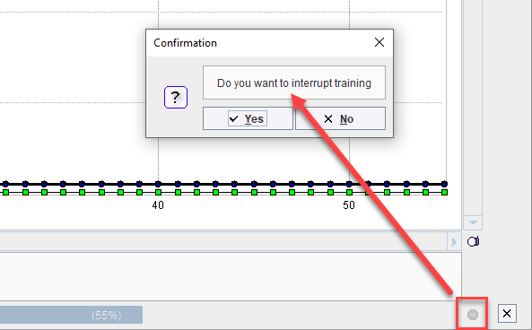
Training may also be stopped by the user. This is useful when training appears to be unsuccessful with no improvement in the loss value or when training has been particularly successful and a plateau in loss value has been achieved with many epochs remaining:
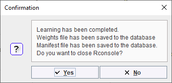
A confirmation dialog in the R Console confirms that learning was completed and the components saved. The R Console can be closed:
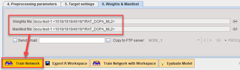
The Weights and Manifest are now attached to the Learning Set:
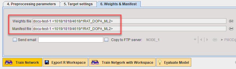
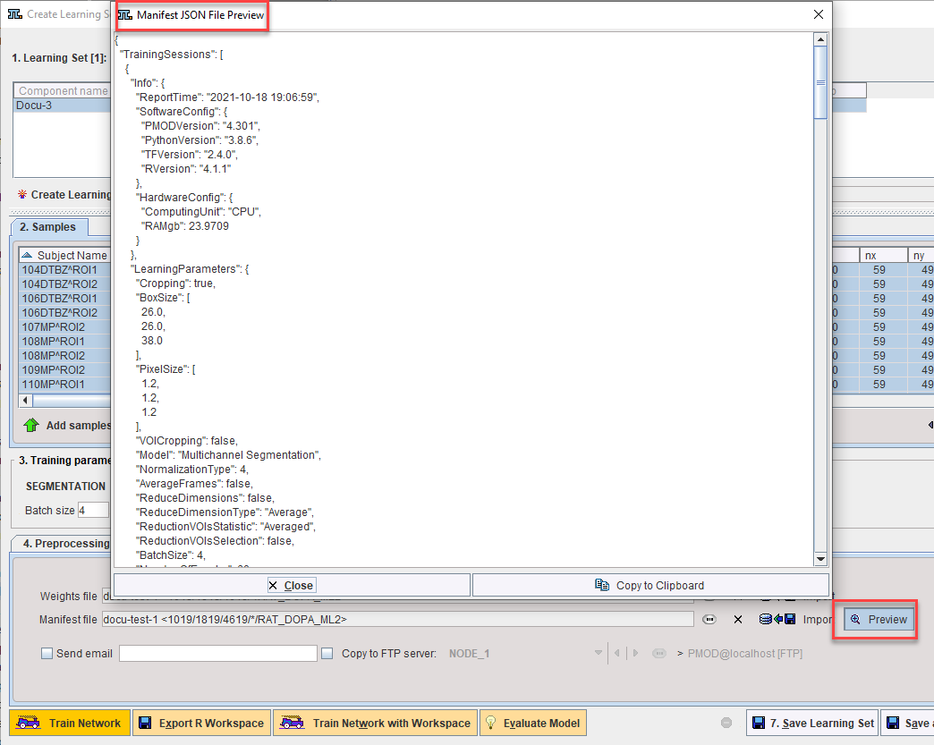
Details of the training are recorded in the Manifest. It can be reviewed using the Preview function on 6. Weights & Manifest:
Additive Training
The best results are achieved by training in a single session with the maximum amount of data available. However, in a situation where the initial number of samples is limited and new samples will become available on a regular basis it is possible to try additive training. For example, where 50 samples are available at the start of a project and 10 new samples will be preprocessed every two weeks.
Additive training is achieved by adding the new samples to your existing Learning Set, selecting a subset of the total Learning Set (a combination of existing samples and new samples is recommended, e.g. select the 10 new samples and 10 existing samples), then launching Train Network based on the existing Weights and Manifest (identified on 5. Weights & Manifest).
Evaluation of the Model
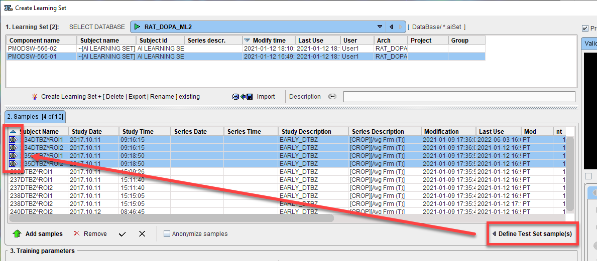
Once the model has been trained, a subset of samples in 2. Samples can be designated as Test Set samples and used as an additional evaluation of the model. Samples can be labeled as Test Set prior to training so that they are excluded for this use in evaluation.
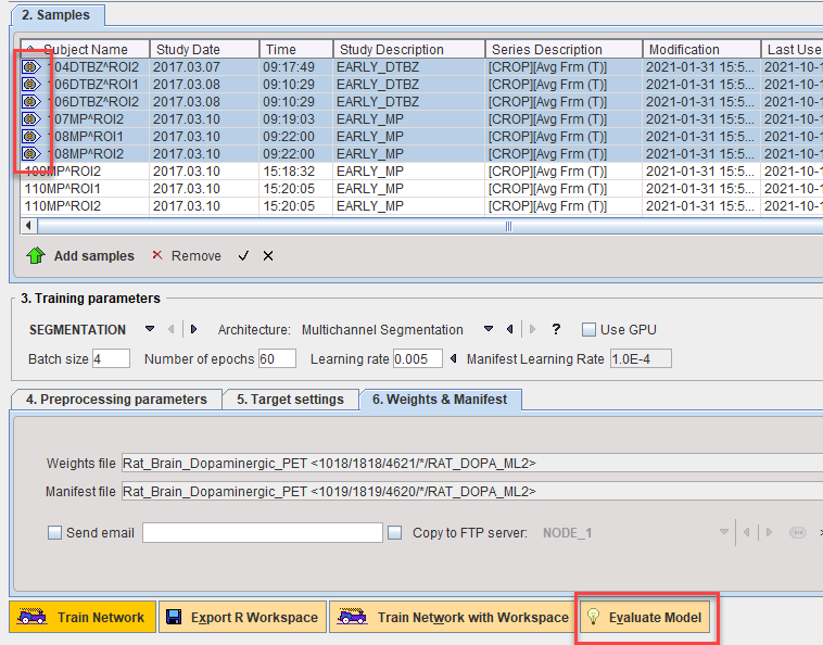
The performance of the model on the Test Set can be calculated using Evaluate Model:
Prediction will be run in R Console and each predicted segment compared to the reference associated with the sample. An average loss value for the test set samples will be returned.