Overview of Ridge-Regression Fitting
Because of the high noise level in pixelwise TACs the fitting of a full 2-tissue compartment model is often not successful. One way to alleviate this problem is to reduce the number of fitted parameters, for instance by fixing the values of k4 and/or K1/k2 at a value which can be reasonably assumed as constant across all tissues. As an example, with PMP, Koeppe et al. [1] fixed k4 at a value of zero and the distribution volume of the non-displacable compartment K1/k2 at a value determined beforehand with a regional TAC analysis.
Another approach (which can be combined with parameter fixing) is to try improving the fitting stability by the introduction of constraints. The 2-Tissue Compartment, K1/k2, RR model implements such an approach called ridge-regression fitting. Basically, ridge-regression fitting works as follows:
1.It determines for each image pixel initial values of the model parameters which are relatively close to the final result.
2.It determines a penalty called ridge factor for changing the individual parameters from their respective starting values. Less stable parameters are subject to a stronger penalty. The ridge factors could also vary spatially, but they are asssumed as constant in this implementation.
3.Using the initial parameters it performs a model fit in each pixel. The adjustment of the model parameters is not only dependent on the difference between the model curve and the pixel-TAC, but also on the difference between the initial and the actual model parameters and their penalties.
CAUTION: While the ridge-regression constraints make fitting more stable, there is a danger that the fit results are biased. For instance, if the penalties are very high, the parameters will not be varied at all, and the fit will return the initial parameters. Therefore, the user should experiment with the ridge factors and compare the results of pixelwise fitting with the results when fitting regional TACs before accepting the pixelwise fitting results.
K-Means Clustering
The initial values of the model parameters are automatically determined by the following approach:
1.Background pixels are removed by calculating the signal energy of the pixelwise TACs (sum of squared TAC values), and considering only pixels above a specified percentile. These remaining pixels are classified into N clusters using a k-means algorithm [2]. The time-weighted Euclidean distance can be used as the measurement of dissimilarity (or distance) between TACs.
2.N non-background pixels serving as initial cluster centroids are randomly assigned.
3.Each pixel is assigned to that centroid with minimal distance between the TACs, thus forming N initial clusters.
4.For each cluster a new centroid TAC is calculated as the average TAC of all pixels in the cluster.
5.An iterative process is started which repeats the following two steps:
(1) Each pixel TAC is compared with all centroid TACs and assigned to the cluster with minimal distance.
(2) All centroid TACs are recalculated to reflect the updated cluster population.
The iterations are repeated until no pixels are re-assigned to a different cluster, or a maximal number of iterations is exhausted.
6.The final centroid TACs are fitted by a standard two-tissue compartment model without penalties, yielding N sets of fit parameters (K1, K1/k2, k3, k4) together with estimates of their standard errors derived from the fitting covariance matrix of the Marquardt-Levenberg algorithm.
Non-Linear Ridge Regression
For the ridge-regression fitting of the pixelwise TACs with a two-tissue compartment model, the standard cost function WRSS (weighted residuals sum of squares) is extended by a term which penalizes the local parameter variation [3,4]. This TSS (total sum of squares) criterion is given by the expression [5]
![]()
where θ denotes the parameter set to be optimized, βi the initial parameter estimates, and hi the ridge factors for the p fitted parameters. This TSS criterion is integrated into the Marquardt-Levenberg optimization, including the calculation of the Hessian and gradient matrices.
For performing the pixelwise ridge-regression fits, for each parameter a βi image is needed which provides a reasonable approximation of the final parameter value. Assuming successful clustering and stable fits of the centroid TACs, βi images are obtained by creating cluster images using the parameter values resulting from the centroid fits, and applying a spatial filter to accommodate smooth transitions. A simple average filter is used which replaces a pixel value by the average within a certain spatial neighbourhood.
The ridge factors hi should be chosen such that changes of unstable parameters are penalized to a stronger extent. Assuming that a large standard error (ste) indicates a parameter which suffers from a high variability, it is included in the ridge factors [3]. To allow more variation for parameters with a large value range across the clusters, the ridge factors are calculated by
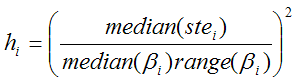
Median(βi) represents the median of the parameter θi across the N cluster fits, and range(βi) the absolute difference between the maximal and the minimal fit value. The ridge factors are smoothed in the same way as the initial parameters. Additionally, the user interface supports a scaling factor for each hi value to allow for manual adjustments of the individual parameter penalties. Finally, the TSS cost funcion is iteratively optimized using the extended Marquardt-Levenberg method.
Overview of the Processing in PXMOD
During Preprocessing, a cluster analysis is performed for suppressing the background and grouping the remaining pixels into clusters of similar uptake over time. Then, a 2-tissue compartment model is fitted without constraints to the average TAC of the clusters. To obtain initial parameter values per pixel, the parameter values resulting from the cluster TAC fits are assembled into parametric maps, which are smoothed. The user should check the clustering and the initial parameter maps to verify that the number of clusters is adequate and the grouping successful. The system also derives estimates of the ridge factors from the fit results, which can be separately scaled by the user.
Since processing of the whole data set will take substantial time, the user should then pixelwise fit (now with ridge regression) a single image slice for confirming that the settings of the ridge factors are suitable. He can do so by comparing the parametric maps of the inital parameters with the result parameters. If there is no change, the ridge factor is too strong; if there are changes but the noise is too high, the ridge factor is too weak. The user should adjust the ridge factors of the individual parameters accordingly, and then try again.
Note that the iterative fitting of all image pixel TACs is a computationally intensive process and may well take hours. For efficiently working with this model it is recommended:
•To make sure background is properly masked to avoid unnecessary, time-consuming fits.
•To first test the model configuration by processing only the current slice (enable the 1S flag).
•Possibly set up a batch and run the fitting with different ridge factor settings over night.
Acquisition and Data Requirements
Image Data |
A dynamic PET data set with 2-tissue kinetics. |
Blood Data |
Input curve from the time of injection until the end of the acquisition. Optionally, whole-blood activity can be used for spillover correction. |
TAC1 |
A time-activity curve (or VOI) of representative tissue used to determine the initial model parameters which are used for the cluster TAC fitting. |
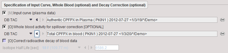
Blood Preprocessing
It is assumed that no reprocessing other than an optional decay correction must be applied to the blood activities. This plasma activity serves as the input curve of the 2-tissue compartment model, and the whole blood activity for spillover correction.
Model Preprocessing
The model preprocessing panel specifies a tissue time-activity curve (TAC1, FILE or VOI), and the parameters a 2-tissue compartment model configuration. Only the parameters which have the fit flag enabled are varied, while the other ones are kept fixed. The user should enter reasonable initial parameter values. They are most easily obtained in the PKIN tool. To transfer the current data quickly to the PKIN tool, just select the kinetic modeling button. Additionally, the dialog window contains parameters related to the clustering and ridge regression fitting.
During Preprocessing the TAC1 is iteratively fitted, and the model parameter values updated accordingly. Then the cluster analysis is performed, the centroid TACs fitted, and the fitting results used for setting up the maps of initial fitting parameters.
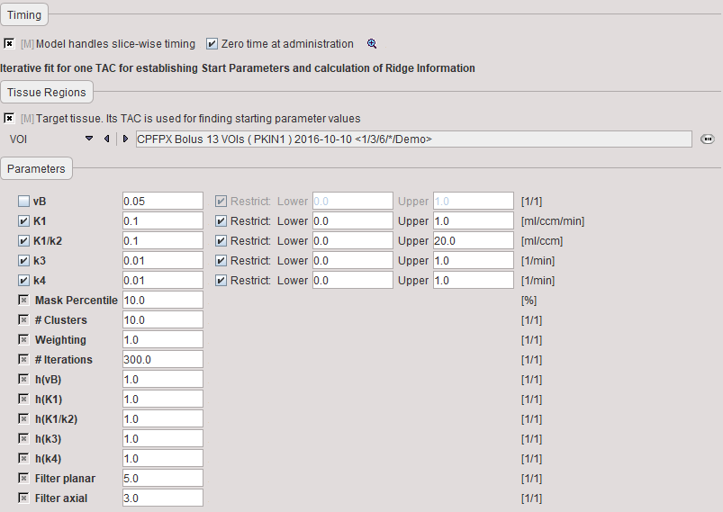
vB |
Blood volume fraction. Is usually fixed at a value of 0.05 representing that 5% of the signal is from the blood space. |
K1, K1/k2, k3, k4 |
Fit parameters of the two-tissue compartment model using the non-specific distribution volume K1/k2 as a fitting parameter instead of k2. They are updated by the results of fitting the model to TAC1. |
Mask Percentile |
To mask out backgound pixels, a map of the TAC signal energy is calculated. The signal energy is the sum of all squared values of a TAC. A histogram analysis is performed, and all pixels which have a signal energy below a specified percentile are considered as background pixels. |
# Clusters |
Number of clusters into which the non-background pixels are grouped. |
Weighting |
During the clustering, the distance between the TACs is calculated as the sum of the squared weighted differences. The valid choices are: |
# Iterations |
Maximal number of refinements during the cluster analysis. Is required to avoid loops. |
h(vB) |
User-defined scaling factor for the ridge factor of the vB model parameter. The behavior is exponential, so entering values of 0, 1, 2, etc result in scaling factors of 1, 10, 100 (10h). Higher ridge factors punish parameter variation. |
h(K1), h(K1/k2), h(k3), h(k4) |
User-defined scaling factors for the other ridge factors as described above. |
Filter planar |
In-plane width of the averaging filter for spatially smoothing the initial parameters. Specification of a planar filter size of 5 and an axial filter size of 3 results in a (5x5x3) averaging filter. |
Filter axial |
Axial width of the averaging filter, see above. |
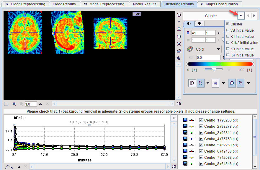
The results of model preprocessing are available on the dedicated Results and the dedicated Clustering Results panels. The Results panel shows the fit to the TAC1 curve together with the parameter values.
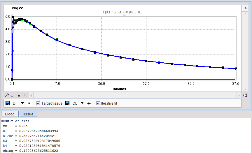
The Clustering Results panels allows inspecting the parametric images of clustering and the initial parameters for the pixelwise fit. The curve area in the lower part shows the cluster centroid TACs, ie the average TAC of all pixels in the cluster.
Model Configuration
The model dialog contains a substantial number of parameters for which maps can be calculated. They are arranged in 3 groups:
1.The actual fit parameters vB, K1, K1/k2, k3, k4 of the 2-tissue compartment model. Note that the same parameters should be enabled for fitting as during the Preprocessing.
2.Parameters which are derived from the fitted model parameters such as the distribution volumes and the flux.
3.The inital values of the model parameters calculated during Preprocessing which are used for pixelwise fitting. They are helpful for assessing to what extent the parameters were adjusted during ridge-regression fitting.
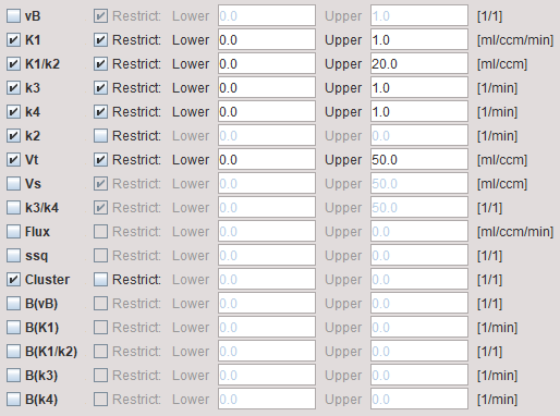
vB, K1, K1/k2, k3, k4 |
The parameters of the 2-tissue compartment model. The fit flag determines, which parameters are actually fitted, and which are fixed. |
k2 |
The k2 rate constant k2 = K1/(K1/k2) |
Vt |
Total volume of distribution: Vt = K1/k2(1+k3/k4) |
Vs |
Distribution volume of specific binding: Vs = K1/k2 *k3/k4 |
k3/k4 |
Binding potential: BPND = k3/k4 |
Flux |
Flux to the second compartment: Flux = (K1k3 )/(k2+k3) |
ssq |
Chi squared of the fit. The corresponding map shows where the fitting was not able to achieve a good match, for instance in pixels of the blood pool. |
Cluster |
Index of the cluster to which the pixel belongs. 0 represents a background pixel. Cluster images could be helpful for VOI analysis. |
B(vB), B(K1), B(K1/k2), B(k3), B(k4) |
Initial values of the model parameters for fitting the 2-tissue compartment model in the individual pixels. |
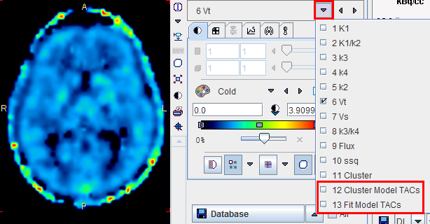
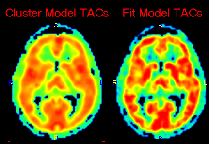
Additional Results: Synthetic dynamic series
In addition to the parametric maps the model also calculates two dynamic image series:
1.Cluster Model TACs: Synthetic image series assembled from the model TAC in each pixel which is calculated using the 2-tissue compartment model and the initial parameters.
2.Fit Model TACs: Synthetic image series assembled from the model TAC in each pixel which is calculated using the 2-tissue compartment model and the fitted parameters.
These image series can serve as phantom images for research, because the uptake in each pixel represents ideal 2-tissue kinetics, and the model parameters are exactly known. So other quantification methods can be applied to analyze these synthetic data and the results compared with the true parameters, which are available as parametric maps.
References
1.Koeppe RA, Frey KA, Snyder SE, Meyer P, Kilbourn MR, Kuhl DE: Kinetic modeling of N-[11C]methylpiperidin-4-yl propionate: alternatives for analysis of an irreversible positron emission tomography trace for measurement of acetylcholinesterase activity in human brain. J Cereb Blood Flow Metab 1999, 19(10):1150-1163. DOI
2.Velamuru PK, Renaut RA, Guo H, Chen K. Robust Clustering of Positron Emission Tomography Data. Paper presented at: Joint Conference of the Classication Society of North America and Interface Foundation of North America, 2005; St. Louis.
3.Byrtek M, O'Sullivan F, Muzi M, Spence M. Use of ridge regression for improved estimation of kinetic constants from PET data. IEEE Trans Nuclear Science. 2005;52(1):63-68.
4.Zhou Y, Huang SC, Bergsneider M, Wong DF: Improved parametric image generation using spatial-temporal analysis of dynamic PET studies. Neuroimage 2002, 15(3):697-707.
5.O'Sullivan F, Saha A: Use of ridge regression for improved estimation of kinetic constants from PET data. IEEE Trans Med Imaging 1999, 18(2):115-125.