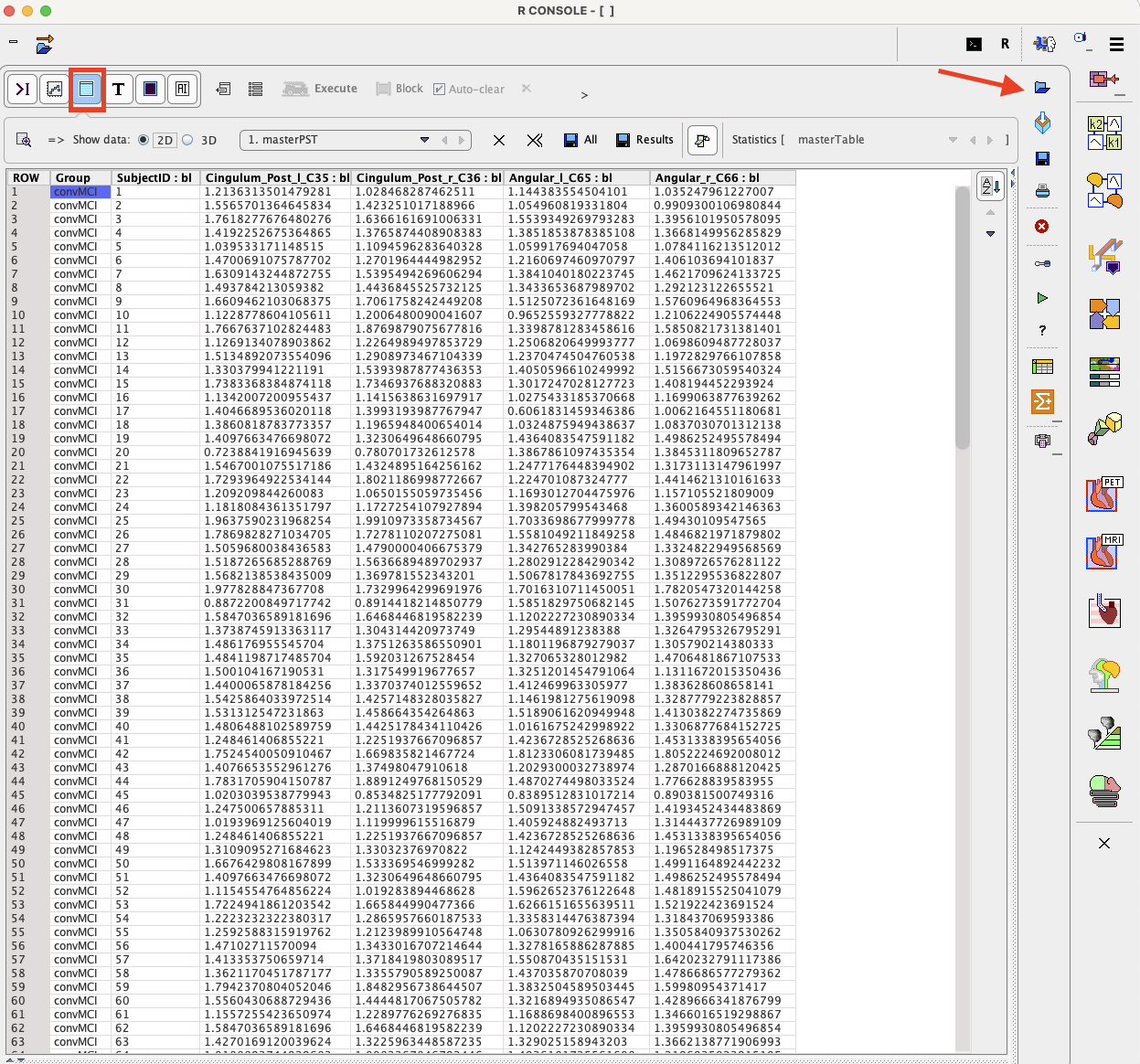
To start the analysis load the example Example_LDA.RData workspace which is available in the Pmod example database. Use the Load/Workspace Data option from the lateral task bar. It already contains the master table which forms the basis for the analysis. To visualize the master table select the Table layout icon as shown below:
To start the analysis please select the Linear discriminant analysis entry in the scripts list:

The linear discrimination interface opens. To select the Master table for the analysis use the selection arrow on the top. Correspondingly, summary of the master table content is shown in the Input data restriction section. Make sure all Groups and VOIs are selected.

The analysis is started with the Ok button.
Logistic regression produces the following output accessible via the Text layout:
1.The summary(lind_glmFit): this indicates that both, left PCC and left angular gyrus contribute significantly to discrimination (p value of 0.01393 and 0.01702 respectively). Interestingly, the right PCC is included marginally (p = 0.065) but with a negative slope estimate, indicating that it is the left/right difference that provides better discrimination than either side alone. The contribution of the right angular gyrus is considered nonsignificant.

2.The stepAIC(fit, direction="backward") is displaying the stepwise procedure to eliminate unneeded predictors progresses. The result indicates that, only removing right angular gyrus improves AIC (smaller values are better), while removing any of the other predictors worsens the fit more (increasing deviance) than the reduction of predictors is worth.

3.The final fit summary(lind_fitAIC_DM) is, with all three remaining regions providing a significant contribution:

4.The lind_fitAIC_DMCoeff is representing the linear coefficients of the discrimination model and is also accessible in the Table layout. This result will be used in the prediction step

The quality of the discrimination can be checked via the Plot layout:

The blue line is respresenting the ROC curve of the full model based on four predictors with an area under the curve (AUC) of 0.7518. The roc.formula in the code is producing the following output:
Call:
roc.formula(formula = GROUP ~ fit$fitted.values, data = columns)
Data: fit$fitted.values in 78 controls (GROUP convMCI) < 129 cases (GROUP MCI).
Area under the curve: 0.7518
The red line is representing the the ROC curve of the final fit based on three predictors instead of four. As to be expected it has a minimally smaller AUC of 0.7486. The roc.formula in the code is producing the following output:
Call:
roc.formula(formula = GROUP ~ fitAIC$fitted.values, data = columns)
Data: fitAIC$fitted.values in 78 controls (GROUP convMCI) < 129 cases (GROUP MCI).
Area under the curve: 0.7486
The script produces a box plot of the master table data selected for the LDA analysis.

The box plot is providing a side by side comparison of the groups and VOIs.
The purpose of the linear discriminant analysis (LDA) in the example above was to find the linear combinations of the original variables (here indicating the FDG concentrations in the ROIs) that gives the best possible separation between the MCI which progress to dementia and those who remain stable. The discriminant function is representing the linear combination of the variables:
t = -4.687+3.994*leftPCC-3.386*rightPCC+2.843*leftAngC
It is recommended to save the LDA results as a workspace using the save icon in the lateral taskbar.