Setup of a Pipeline per Group/Condition
1.Configure the processing steps of the pipeline. After testing its performance with some example data, remove all files from the list and save it as the processing template with Save Processing.
2.Configure a meaningful set of input files (e.g. control group, baseline scans) in the List of Input Studies. Use Save processing for saving this processing batch. In the dialog window
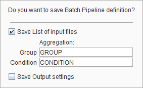
enable Save List of Input files so that the currently selected files are stored together with the processing definition. In order to prepare aggregating the VOI statistic or kinetic parameters of this batch into an overall table specify the Group and the Condition identifiers in the corresponding fields (e.g. "Control" and "Baseline"). Choose a corresponding name for the file and save.
3.Remove all input files, then configure the next set of input files (e.g. control group, follow-up scan). Save the processing list as in 2. with appropriate aggregation information (e.g. "Control" and "Follow-Up".
4.Repeat 3. for all subject groups and conditions (e.g. "Patient", "Baseline"; "Patient", "Follow-Up"). Make sure to use consistent identifier names.
List of Pipelines
For setting up an overall batch processing load all the prepared pipelines into the List of Pipelines tab using the Set processing files and Add files buttons.
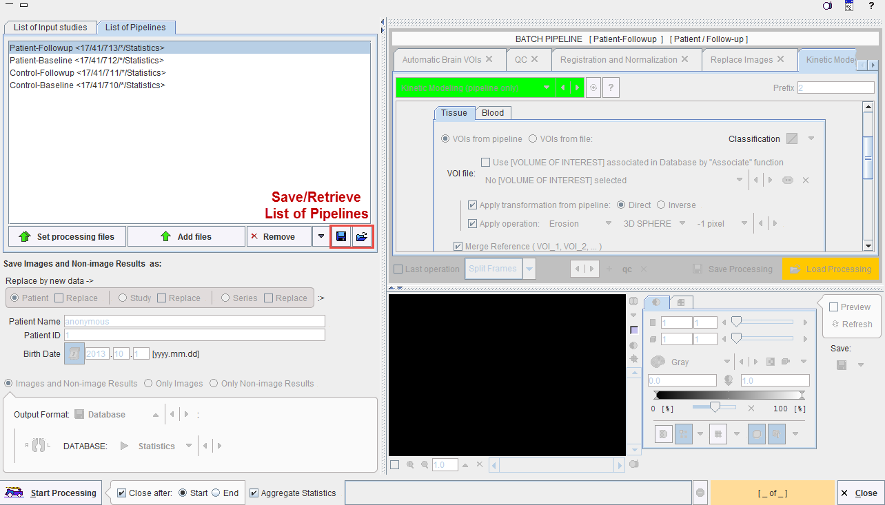
The Aggregate Statistics option enables the creation of an aggregate per pipeline, which summarizes the group results and is named according to the Group and Condition identifiers. Note the functionality for saving the whole definition and retrieving it at a later time.
Execution of Pipelines List
After setting the pipelines up or retrieving them, the batch can be launched with Start Processing. A dialog window appears which summarizes the tasks to be performed
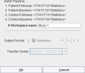
and allows defining an R Workspace name. This is a convenience and only relevant if the R functionality is enabled. In that case, all group aggregates are imported into the R environment and saved as a workspace, which can directly be employed for the population analysis.
The example below illustrates the situation at the end of processing the configuration above: Four aggregates were created, transferred to the R console which automatically started, and the interface for the population statistics is opened.
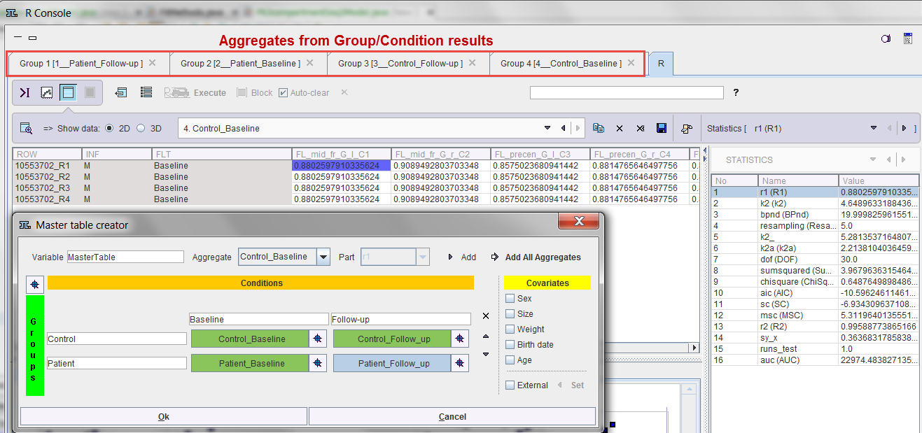
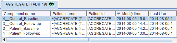
The individual pipeline aggregates are also available and appear as the following entries in the database.