The PVC (Brain MR based) method implemented in PMOD consists of the following steps:
1. Segmentation of the Anatomical MRI
To perform the segmentation, a normalization transform of the subject MRI anatomy to the MNI anatomy (or space) is calculated. In the MNI space, there are probability maps available for grey matter (GM), white matted (WM) and cerebrospinal fluid (CSF).
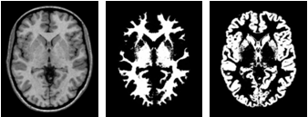
These priors are inversely transformed to the MRI space and employed in the image segmentation. The results are three probability images in the MRI space, called the GM, WM and CSF segments. They form the basis for the PVC.
2. Matching of the PET and MR Images
In order to perform the PVC, the information of the MRI and the PET must be aligned. Because the GM segments are relatively fine, they cannot be resampled to a typical PET resolution without severe information loss. Therefore, the PET image is rigidly matched to the MRI, and the PVC performed in the MRI space on the up-sampled PET images.
3. Partial-volume Effect Correction
First, the uptake in WM is obtained either by analyzing the PET uptake in pixels with very high WM probability, or by using a value provided by the user. Then, the following correction formula of Muller-Gartner is applied:
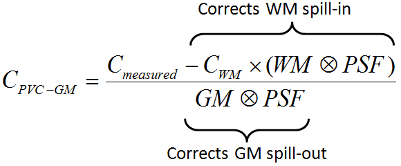
with the following notations:
CPVC-GM |
Corrected activity concentration. This is the result of the PVC correction in each GM pixel. |
Cmeasured |
Actually measured activity concentration in a GM pixel which may be distorted due to spill-out and spill-in. |
CWM |
Activity concentration in WM which is assumed to be homogeneous and just blurred by the PSF. |
WM, GM |
WM (GM) segment image which represents the WM (GM) probability of each pixel in the image as a value between 0 and 1. These images are assumed to represent the true anatomy with ideal resolution. |
PSF |
Point-spread function of the imaging system which is assumed to be constant across the image and represented by a three-dimensional Gaussian function. |
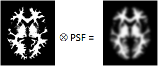
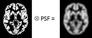
WM⊗PSF |
Mathematical convolution of the WM segment image with the PSF. The result represents the image of the ideal WM segment when detected with a real imaging system characterized by the PSF function.
The expected WM image is obtained by scaling WM⊗PSF by the WM concentration CWM. It is subtracted from the measured image to compensate for spill-in from WM to GM. |
GM⊗PSF |
Mathematical convolution of the GM segment image with the PSF.
A division of the WM-corrected image by GM⊗PSF represents a deconvolution operation and corrects for the spill-out effect from GM. The operation of division may introduce over-corrections at the GM boundary. Therefore, the result image is masked at a certain threshold of the convolved GM image |
Spill-out Correction Only
If, however, the segmentation of white and grey matter fails, the correction can be reduced to a spill-out only correction. In this case a Brain segment is formed from all pixels which are not CSF. This segment is convolved with the PSF, and the PET image divided by the result as described by the equation below.
![]()
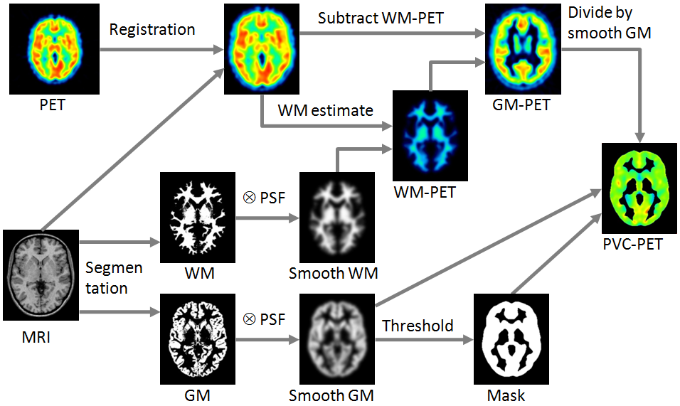
Schematic of the Correction Workflow
The following illustration provides a graphical overview of the different processing steps as well as the resulting intermediate images.