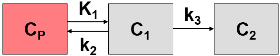
The Patlak plot has been developed by Patlak et al. [1] for tracers undergoing irreversible trapping. Most often it is applied for the analysis of FDG, which can be modeled as a 2-tissue compartment model with k4=0.
However, this model structure is not necessary for the application of the method. It is sufficient to have any compartment in the system which binds irreversibly.
Operational Model Curve
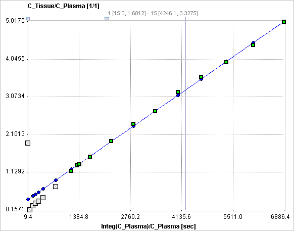
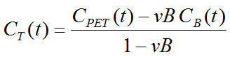
The Patlak plot belongs to a group of Graphical Analysis techniques, whereby the measured tissue TAC CT(T) undergoes a mathematical transformation and is plotted against some sort of "normalized time". The Patlak plot is given by the expression

with the input curve Cp(t). This means that the measured PET activity is divided by plasma activity, and plotted at a "normalized time" (integral of the input curve from the injection time divided by the instantaneous plasma activity). For systems with irreversible compartments this plot will result in a straight line after an equilibration time t*.
The slope K and the intercept V must be interpreted according to the underlying compartment model. For the FDG model mentioned, the slope K equals K1k3/(k2+k3) and represents the metabolic flux, while the intercept V equals V0+vB with the distribution volume V0 of the reversible compartment C1 and the fractional blood volume vB.
Note that an explicit blood volume correction is available via the vB input parameter. In the case of vB=0 (default setting), no correction is performed. For vB>0, the tissue TAC is corrected by the scaled whole blood activity before the actual analysis.
Parameter Fitting
The Patlak Plot model calculates and displays the transformed measurements as described by the formula above. It allows fitting a regression line to the data segment starting at time t*. The results are the Slope and the Intercept of the regression line.
t* can be specified manually, or a value estimated using an error criterion Max Err. For instance, if Max Err. is set to 10% and the fit box of t* is checked, the model searches the earliest sample so that the deviation between the regression line and all measurements is less than 10%. Samples earlier than the t* time are disregarded for regression and thus painted in gray. Note that t* must be specified in real acquisition time, although the x-axis units are in "normalized time". The corresponding normalized time which can be looked up in the plot is shown as a non-fitable result parameter Start. In order to apply the analysis to the same data segment in all regions, please switch off the fit box of t*, propagate the model with the Copy to all Regions button, and then activate Fit all regions.
For the analysis of FDG data, the Lumped Constant (LC) and the Plasma glucose level (PG) of the patient should be entered. The metabolic rate of glucose MRGlu is then obtained from the regression slope by
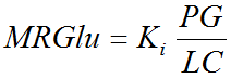
Note: The unit conversion is based on an assumed tissue density of 1.04g/ml.
Reference:
1.Patlak CS, Blasberg RG, Fenstermacher JD: Graphical evaluation of blood-to-brain transfer constants from multiple-time uptake data. J Cereb Blood Flow Metab 1983, 3(1):1-7. DOI