Coupled Fitting to Estimate and Apply a Common k2'
The following sequence of steps is recommended for coupled fitting. The example illustrates fitting of a common k2' using the SRTM2 model. It is equivalent to the SRTM model, but due to a different arrangement of the equations k2' appears as a fitting parameter which allows using coupled fitting.
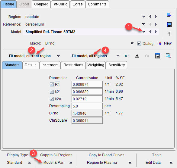
1.Select a regional TAC with good signal.
2.Switch to the model (SRTM2) to be applied in coupled fitting.
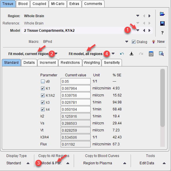
3.Fit the TAC with Fit model, current region and propagate the model to all other regions with the button Model & Par. Use Fit model, all regions to establish model and reasonable starting values for all TACs.
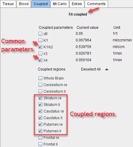
4.On the Coupled panel, enable the parameter(s) which are to be treated as common, and enable all target regions which should be fitted together. Note that the non-coupled parameters will be estimated per region.
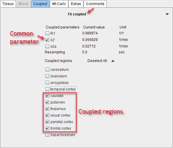
5.Start processing with Fit coupled. Coupled fitting may take significant processing time. Thus the Batch Mode facility may be a helpful option to run such jobs at less busy times.
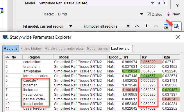
6.On the Tissue panel, switch to one of the coupled regions. The k2' shown there is the common estimate. This can be verified by opening the parameter explorer as below.
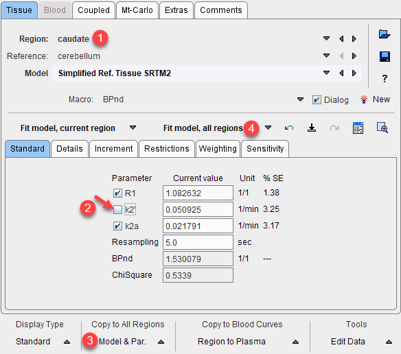
7.To use the common parameters for the fitting in all regions select one of the coupled regions. The Standard panel shows the result of the coupled fit including the estimated values of the common parameters. Note their standard error %SE which should be decreased compared with individual fits. Disable the fit box of the common parameter(s) and propagate this configuration to all regions with the Model & Par button. Apply Fit model, all regions to re-fit the model with the fixed common k2' parameter which is now enforced in all regions.
Coupled Fitting to Improve Robustness of 2-Tissue Compartment Model (2TCM) Fitting
It is often difficult to get robust estimates for k3 and k4 with 2TCM fitting. In order to support parameter coupling, an alternative formulation of the 2TCM is supported which uses K1/k2 (distribution volume of non-displaceable compartment) as fitting parameter instead of k2.
To perform 2TCM coupled fitting proceed similarly as described above:
1.Select a regional TAC with good signal.
2.Switch to the model (2 Tissue Compartments, K1/k2) to be applied in coupled fitting. Fit the TAC with Fit model, current region and propagate the model to all other regions with Model & Par. Fit model, all regions to establish reasonable starting values for all TACs.
3.On the Coupled panel, enable the parameter(s) which are to be treated as common, and enable all target regions which should be fitted together. Note that the disabled parameters will be estimated per region.
4.Start processing with Fit coupled.
5.To use the common parameters for fitting all regions please proceed as described for the common k2' example above.
Coupled Fitting Procedure
The coupled fitting process works as follows:
▪A global target curve is created by stacking the TACs of the checked regions (valid points only).
▪The corresponding weights are calculated according to the weighting configuration for each TAC.
▪A table of fitted parameters is formed by entering the common parameters once and adding all the other fit enabled parameters in the coupled regions. The initial values of common parameters are taken from the first checked region, for the other parameters from the individual regional models. If Float blood parameters is enabled on the Extras pane, the fit-enabled parameters of the blood curves are also taken into account. As a convenience there is a button Fit coupled and delay
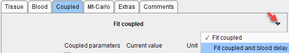
to estimate a blood delay which considers the information from all coupled regions.
▪The optimizer calculates the model curve in all checked regions, creates the global result curve corresponding to the target curve, weighs all the residuals and forms the global sum of squares as the figure of merit. The parameters are adjusted until the cost function has been minimized, and the resulting parameters are copied back to the individual models.