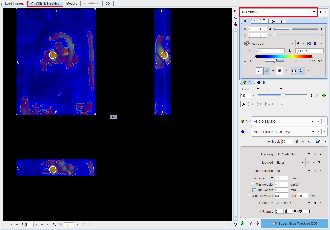
When arriving at the TRACKING page, the image area shows a fusion of the Angio image (A) and the masked Angio image for highlighting areas with high flow. Also shown in the overlay are the VOIs.
Tracking Configuration
The area in the lower right serves for defining the tracking algorithm and its parameters. Two types of tracking options are available for selection:
1.STREAMLINE: is a curve that is instantaneously tangent to the velocity vector of the flow. It shows the direction in which a massless fluid element will travel at any time point.
2.PATHLINE: is a trajectory that an individual fluid particle follows. It can be thought of as recording the path of a fluid element over a certain period. The direction the path takes will be determine by the streamlines of the fluid at each moment in time.
Two algorithms are supported for any of the tracking option and can be selected in the Method list:
1.EULER: Tracking proceeds using a fixed step size along the local fiber orientation [2]. With nearest-neighbor interpolation, this method may be very similar to FACT, except that the step size is fixed, whereas FACT steps extend to the boundary of the next voxel (distance variable depending on the entry and exit points to the voxel).
2.4th order Runge-Kutta method [2]. The step size is fixed, however the eventual direction of the step is determined by taking and averaging a series of partial steps. Interpolation determines how the fiber direction is determined at a given point in space.
The Interpolation setting is not relevant for FACT. For EULER and RK4 the choices are
1.NN: Nearest-neighbor interpolation using the local voxel data directly.
2.NC: Probabilistic nearest-neighbor interpolation, similar to the method proposed by Behrens et al [3]. The data is not interpolated, but at each point one of the 8 voxels neighbors is randomly chosen. The probability of choosing a particular voxel is based on how close the point is to the center of that voxel.
3.TRILINEAR: Linear interpolation of the vector components using the 8 neighbors.
Further parameters and options determine how tracking proceeds and when it ends:
Step size |
Distance between points on the streamlines. Not used for FACT as it does not apply interpolation. |
Min velocity |
Track ends if the velocity amplitude drops below this threshold. |
Min length |
If checked, streamlines/pathlines shorter than the minimal length specified are discarded. |
Max curvature |
If checked, streamlines/pathlines are terminated in case the curvature exceeds the specified angle within the length specified. If length = 0.0, the curvature is checked at each step. |
Colour by |
The streamlines can be functionally colored as follows: |
Frames
|
Tracking is relatively time-consuming. With the box enabled it can optionally be restricted to a certain section of the acquisition. |
Masking
An additional means for restricting the generated streamlines/pathlines is by checking the Mask box and defining a mask. The elements in
![]()
have the following functionality:
|
Generate a mask from the ANGIO STATIC image by applying the specified threshold and include it in the image list B for viewing. |
|
Open the current mask in the VOI editor and convert it into a VOI. The VOI can be edited, and the mask finally updated from the VOI. |
|
Select an external mask file. |
Note: Please first perform tracking without masking, and only afterward gradually increase masking, if necessary.
After configuring all tracking parameters, please proceed with the blue action button. Based on the selected Tracking option, the streamlines or the pathlines are calculated and visualized on the 3D page.
References
1.Mori S, Crain BJ, Chacko VP, van Zijl PC: Three-dimensional tracking of axonal projections in the brain by magnetic resonance imaging. Ann Neurol 1999, 45(2):265-269.
2.Basser PJ, Pajevic S, Pierpaoli C, Duda J, Aldroubi A: In vivo fiber tractography using DT-MRI data. Magn Reson Med 2000, 44(4):625-632.
3.Behrens TE, Woolrich MW, Jenkinson M, Johansen-Berg H, Nunes RG, Clare S, Matthews PM, Brady JM, Smith SM: Characterization and propagation of uncertainty in diffusion-weighted MR imaging. Magn Reson Med 2003, 50(5):1077-1088. DOI