The example is from a study by Varnas et al. [9], who actually used a LME model for the analysis of their data. A new PET ligand for 5HT1B receptors was tested once at baseline, twice under medication with zolmitriptan, and once more after 1 week free of medication. Complete data were acquired in 5 normal volunteers. Binding potentials (BP) were analyzed in two large regions of interest (VOIs), occipital cortex (OCC) and the rest of cerebral cortex (CC). A master table of BP was constructed containing the two VOIs at 4 time points (BL, T1, T2, T3) in 5 individuals.
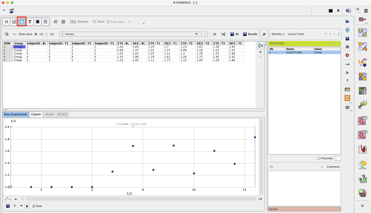
To start the analysis load the example Varnas_LME.RData workspace which is available in the Pmod example database. Use the Load/Workspace Data option from the lateral task bar. It already contains the master table which forms the basis for the analysis. To visualize the master table select the Table layout icon as shown below:
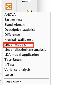
To start the analysis please select the Linear models entry in the scripts list:
The content of the master table is summarized.
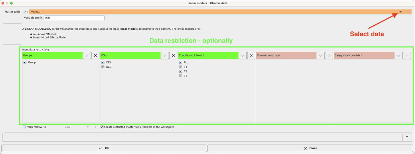
Confirm the setting with the Ok button. The program analyses the content of the "restricted" master table and provides a summary of the analysis and the suggestion for the linear model to be applied. When a single group is studied in different conditions only the linear mixed effects (LME) model can be used for the analysis. Therefore, the selection is blocked and set to Linear Mixed Effects Model:
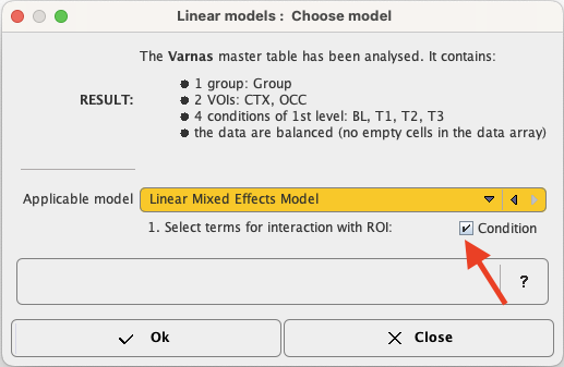
Please note that additional settings are available for the LME: the interactions. The number of available interactions depends on the number of factors and covariates in the master table. To consider an interaction enable the corresponding checkbox. In the example above the interaction ROI:Condition is enabled. Start the analysis with Ok.
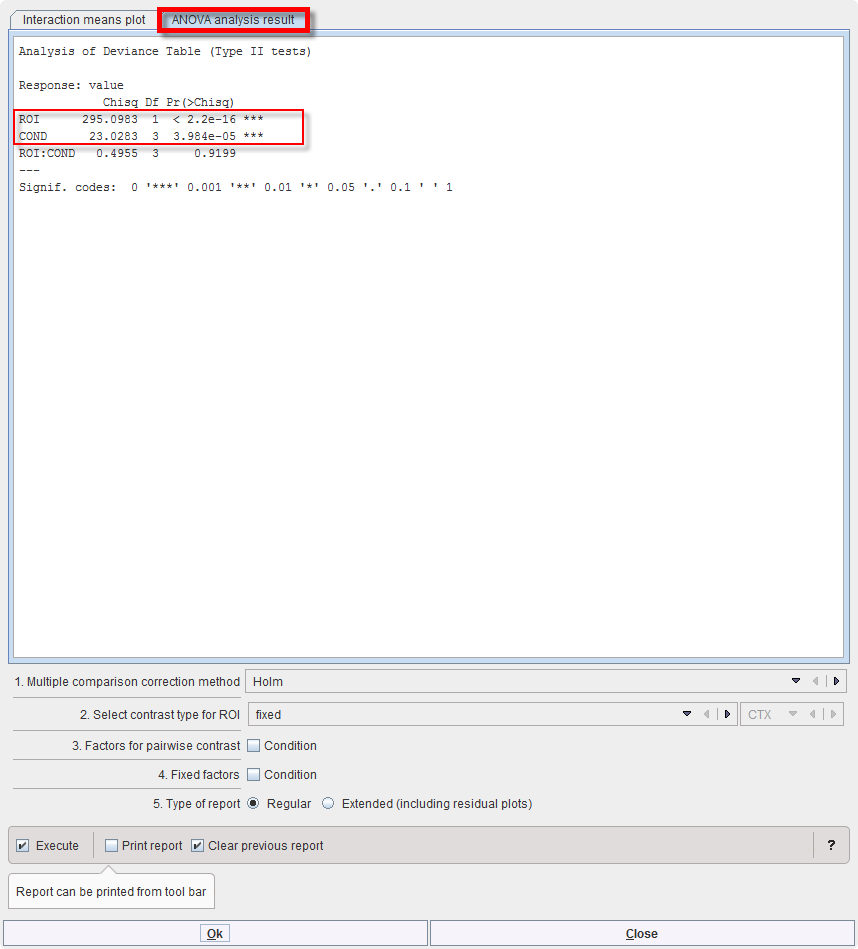
The MANOVA preliminary results indicate that, as an expected trivial result, BP differs between the two regions. More interestingly, it is also significantly differs between conditions. There is no ROI:COND interaction – thus, both regions respond in a similar way to the conditions:
As for MANOVA, “interactionMeans” (R package “phia”) provides an informative graph of the mean effects and their interactions. It demonstrates higher values for region OCC than CTX (top left), which is actually the case under all 4 conditions (bottom left). The last measurement (T3) tends to be higher than the previous ones (bottom right), and that is evident in both regions (top right):
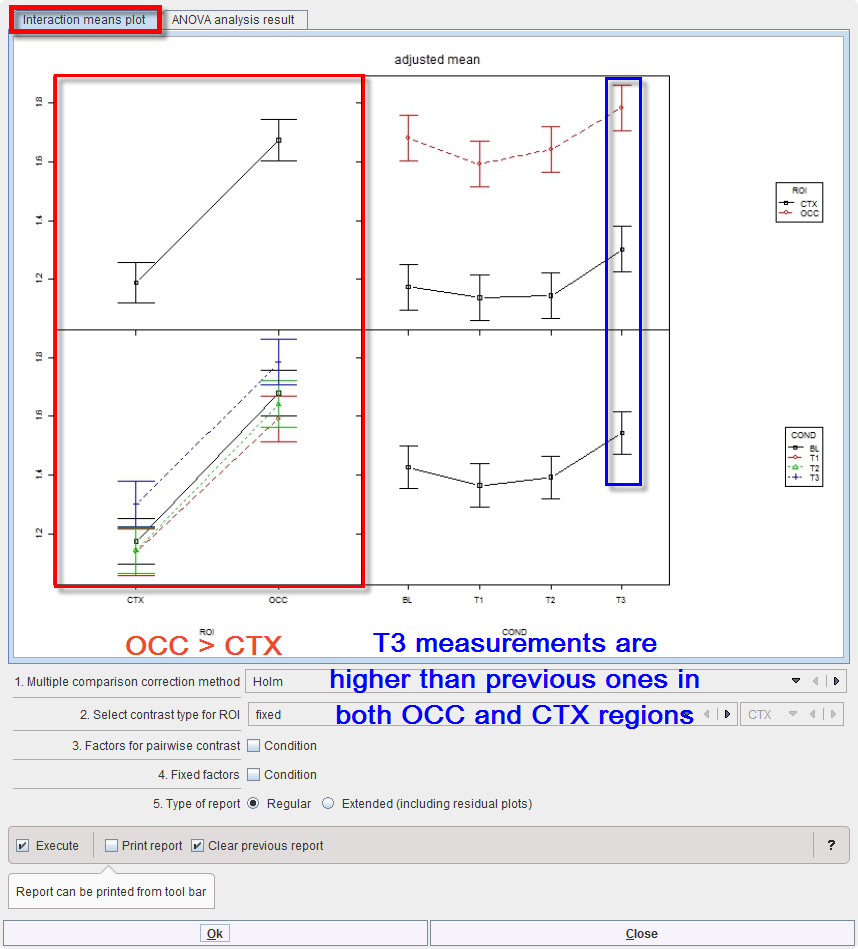
The off-diagonal panels show the first-order interaction means for each pair of factors. The lack of parallelism between lines reveals how one factor changes the other one. The diagonal panels represent the marginal means of each factor.
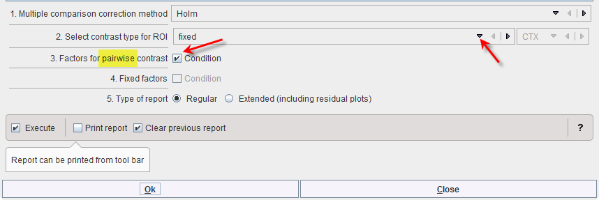
From this graph and the Deviance Table above, the difference between the two regions is clear, but we still are interested in the significance of the pairwise differences between the conditions. We therefore select the appropriate contrasts: “fixed” for ROI and “pairwise” for COND, also using the default correction “Holm” for multiple comparisons:
The result, provided by routine “testInteractions”, is shown in the Text layout:
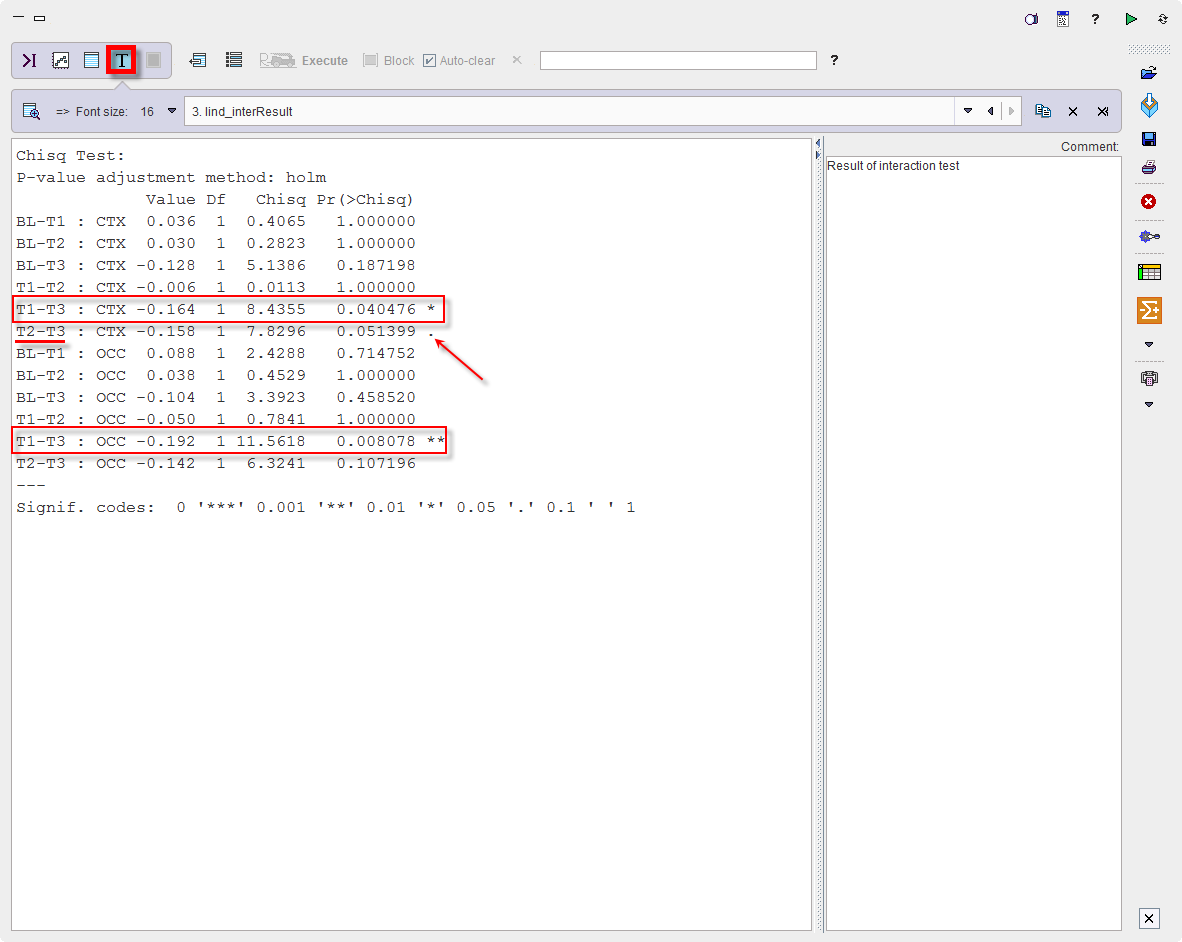
In both regions, a significant difference is present between T3 and T1, with the BP being higher 1 week after stopping the medication (T3) than after its start (T1). A similar tendency is seen for T3 versus T2, while the other differences are far from significance. In that study, this was a somewhat unexpected result suggesting receptor upregulation after medication, requiring further research.
To save the results activate the report button ![]() in the lateral taskbar.
in the lateral taskbar.